Counting Solution with SageMaker Object Detection Built-in Algorithm

Object detection algorithms can be effective for counting objects, and SageMaker has some built-in algorithms. This post describes how to use it through the following steps:
- Labeling images using Ground Truth
- Training and deploying your models
- Performing inference
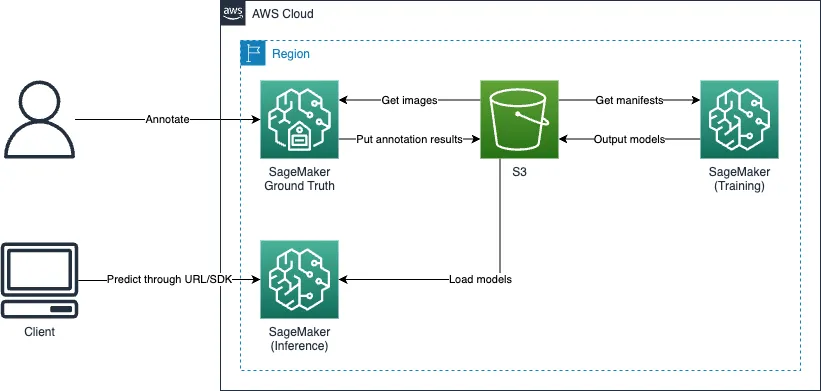
Overview
In my personal opinion, users should not use SageMaker inference endpoints directly for production workloads. This post uses it for testing only.
Labeling using Ground Truth
Ground Truth offers the labeling feature.

Creating Labeling Job
Create your labeling job by following the steps below.
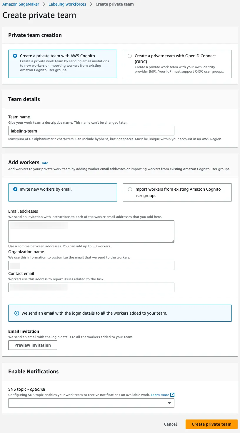
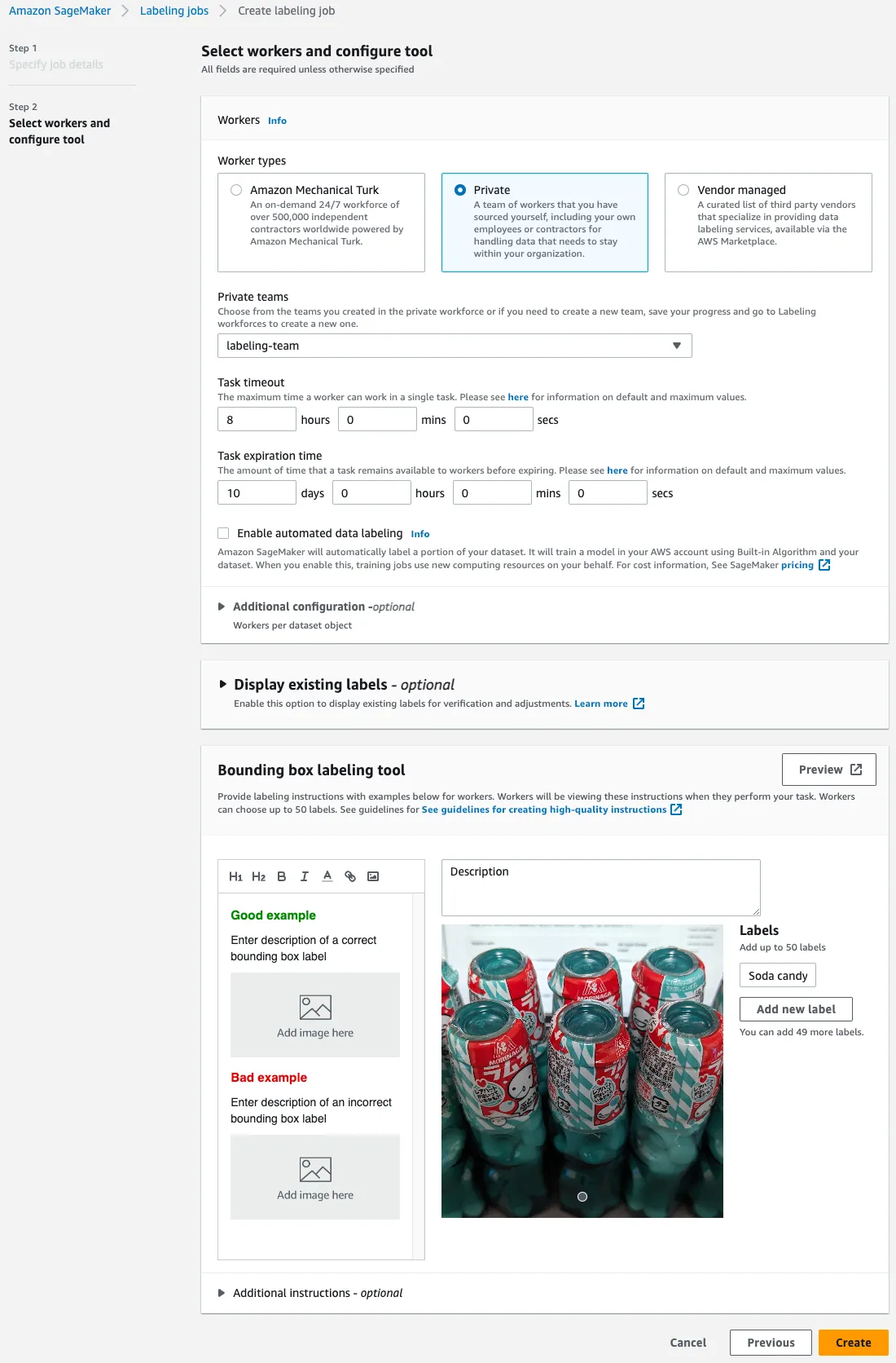
Creating Labeling Workforces
First of all, create your labeling workforces. A private team will be created in this post. Team members can be also authenticated with either Cognito or OIDC.
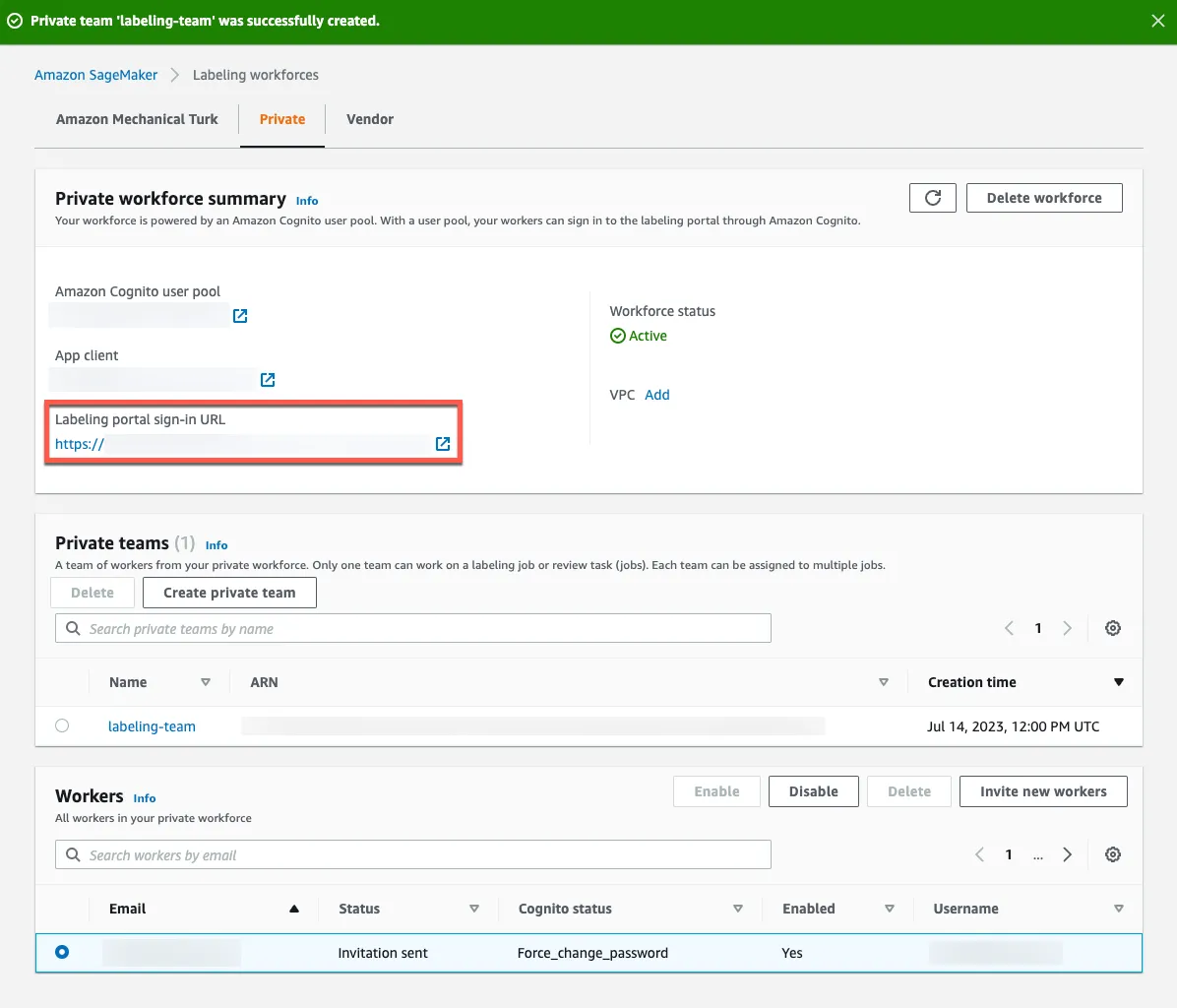
An invitation email has been sent to workers, which displays the labeling portal URL. They can sign up and sign in to the labeling portal using that URL. You can also find the URL, navigating to Private workforce summary > Labeling portal sign-in URL on the management console.
Signing up and Signing in to Labeling Portal
Workers need to sign up and sign in to the labeling portal using information provided in the invitation email.
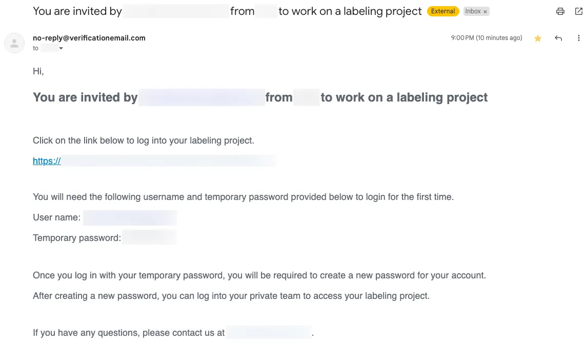
Hi,

You are invited by [email protected] from <COMPANY> to work on a labeling project

Click on the link below to log into your labeling project.
"https://<LABELING_PORTAL_URL>"

You will need the following username and temporary password provided below to login for the first time.
User name: <USER_NAME>
Temporary password: <PASSWORD>

Once you log in with your temporary password, you will be required to create a new password for your account.
After creating a new password, you can log into your private team to access your labeling project.

If you have any questions, please contact us at [email protected].
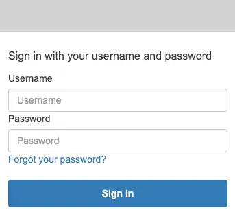
After accessing the URL, enter the username and password in the invitation email.
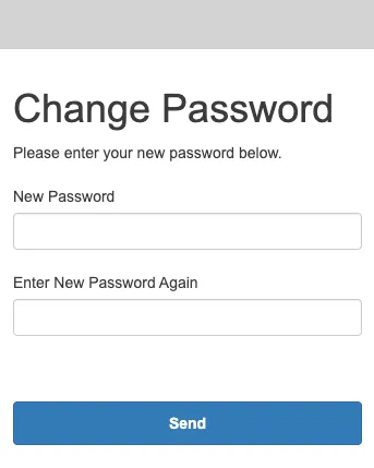
Change the temporal password.
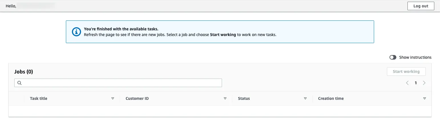
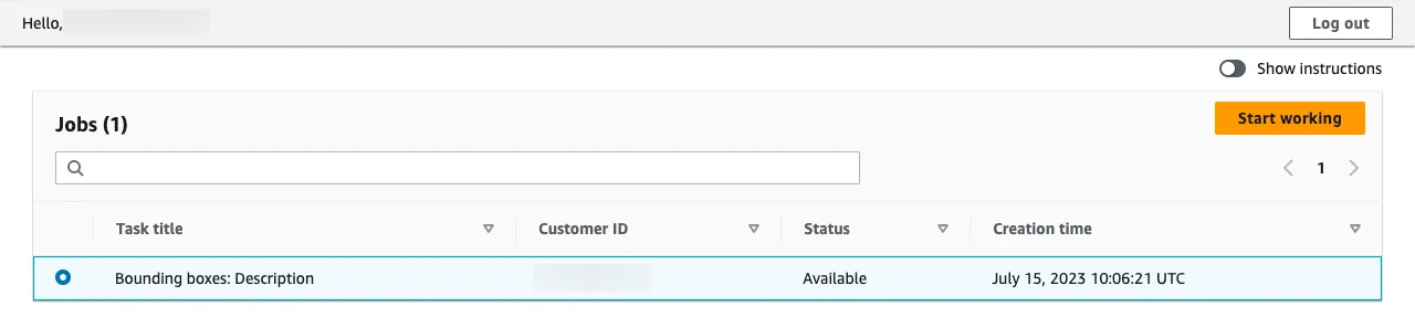
You will be redirected to the top page. On this page, assigned labeling jobs are listed if available.
Creating Labeling Job
Navigate switch back to SageMaker management console, start creating labeling job and enter the field values according to the image below. After creating, the labeling job cannot be deleted, so it is better to use the unique value such as one generated uuidgen | tr "[:upper:]" "[:lower:]". Please make sure to click Complete data setup.
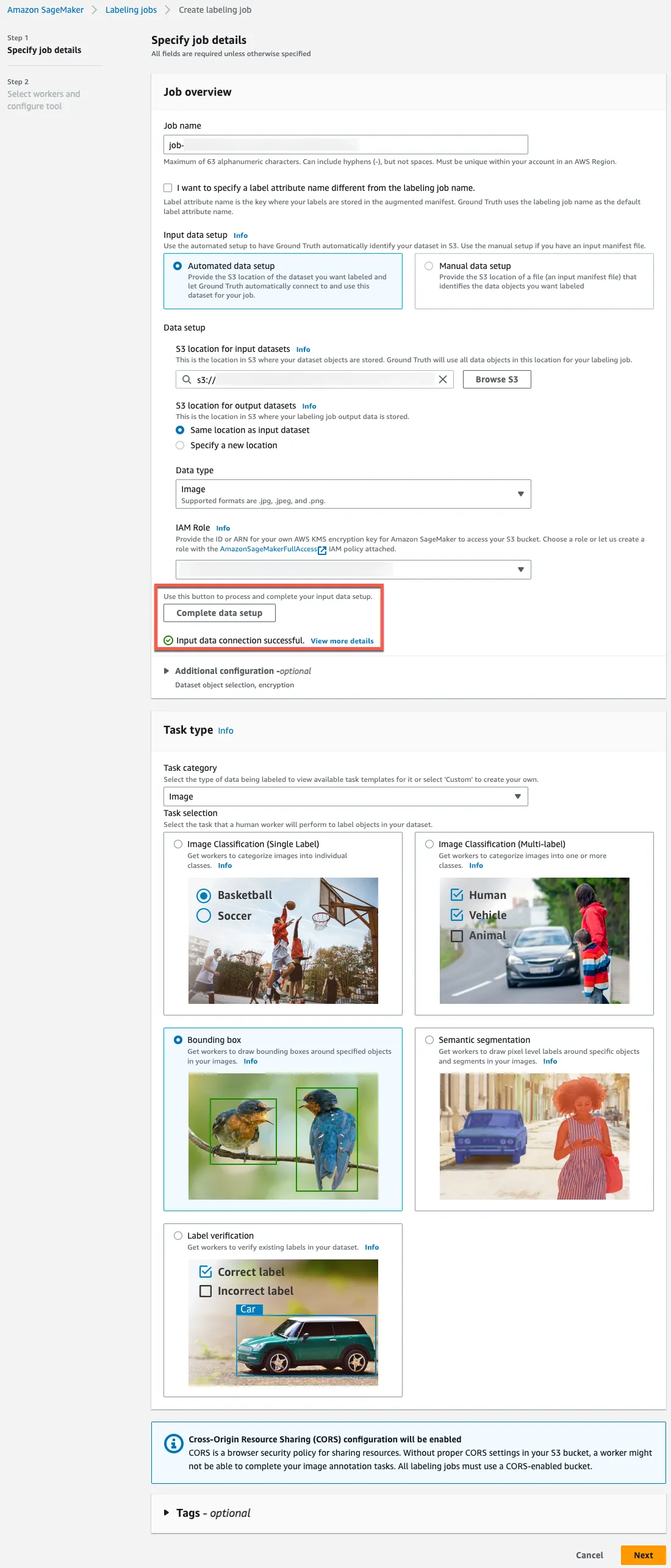
When dealing with complex labeling tasks, it may be better to specify a longer value for Task timeout.
Start Labeling
After signing in to the labeling portal, you should see the labeling job that has been created above. Click the Start working button.
According to the job instructions, label the dataset. Here is the example.
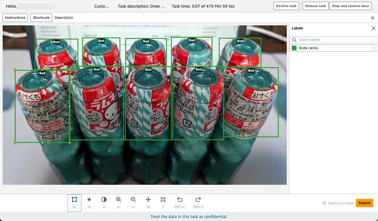
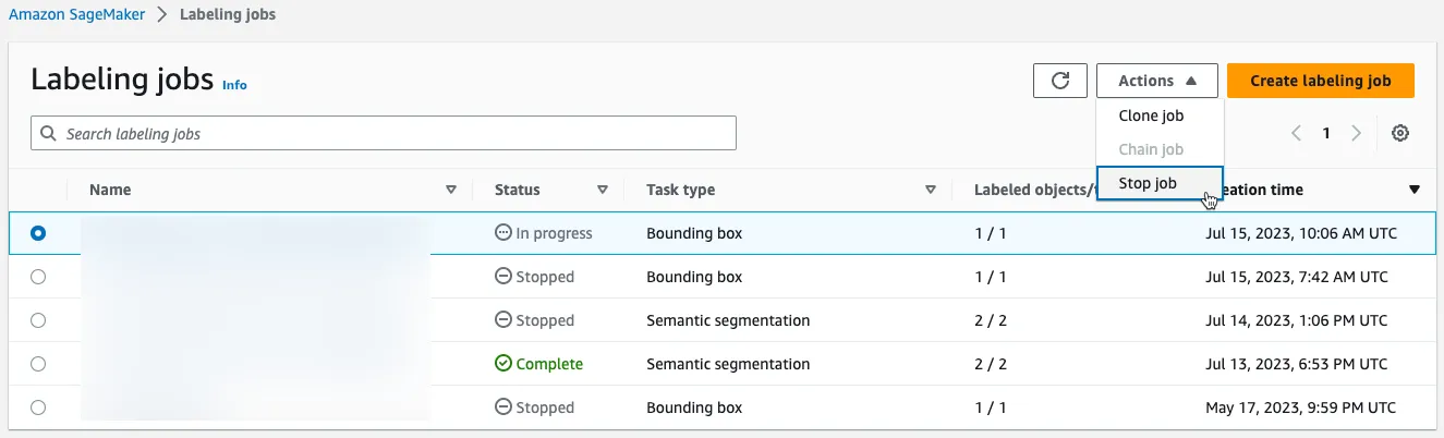
Once all workers have completed the labeling job, stop the job.
Labeling Output
Directories
After stopping the labeling job, its final output has been generated in the specified S3 bucket. For the object detection tasks, manifests/output/output.manifest is important.
<YOUR_OUTPUT_PATH>/
|-- annotation-tool/
|-- annotations/
|   |-- consolidated-annotation/
|   `-- worker-response/
|-- manifests/
|   |-- intermediate/
|   `-- output/
|       `-- output.manifest
`-- temp/
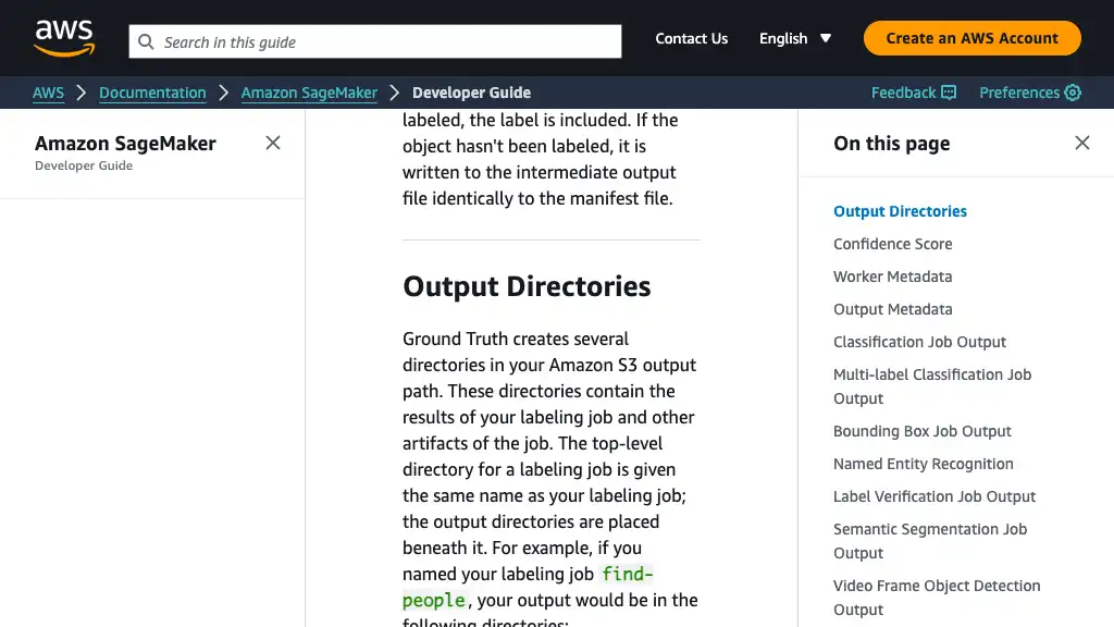
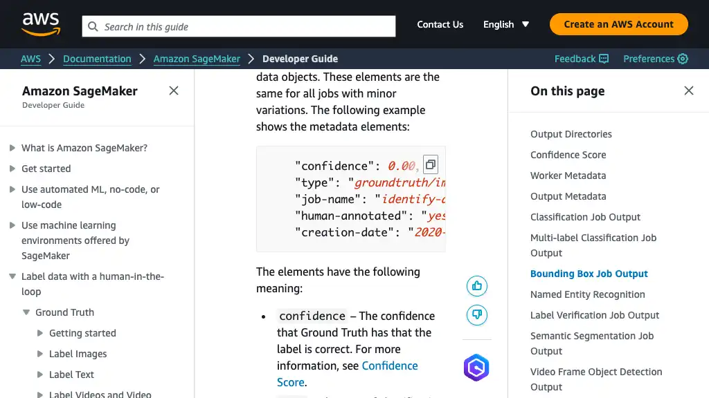
Ground Truth generates labeling results by Augmented Manifest format. Please refer to the official documentation for more details.
Training using SageMaker
Training
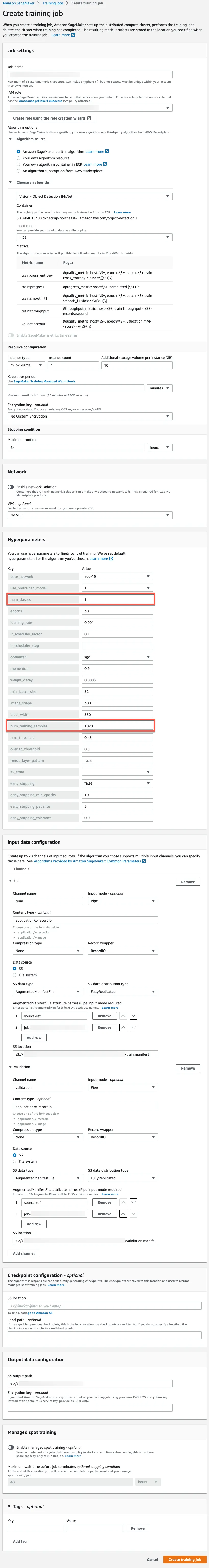
Once the labeling has been completed, train your model using SageMaker console.
The important fields are the following:
- Job settings
- Job name
- The training job cannot be deleted after creation, so it is better to use the unique value such as one generated
uuidgen | tr "[:upper:]" "[:lower:]".
- The training job cannot be deleted after creation, so it is better to use the unique value such as one generated
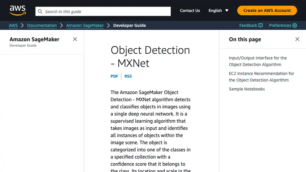
- Algorithm options
- Algorithm source: Amazon SageMaker built-in algorithm
- Choose an algorithm
- Vision - Object Detection (MXNet)
- Input mode: Pipe
- Resource configuration
- Instance type
ml.p2.xlargein this post- Only GPU instances support object detection algorithms.
- Instance type
- Job name
- Hyperparameters
- num_classes:
1in this post - num_training_samples: Count equal to the manifest lines
- num_classes:
- Input data configuration
- train
- Channel name:
train - Input mode:
Pipe - Content type:
application/x-recordio - Record wrapper:
RecordIO - Data source
- S3
- S3 data type:
AugmentedManifestFile - S3 data distribution type: FullyReplicated
- AugmentedManifestFile attribute names
source-ref- Key name containing bounding boxes data
- S3 location: S3 URI of your augmented manifest file for training
- S3 data type:
- S3
- Channel name:
- validation
- Channel name:
validation
- Channel name:
- train
- Output data configuration
- S3 output path: S3 URI of your model artifacts which SageMaker produces
Thanks to the augmented manifest file generated by Ground Truth, we can use Pipe input mode and RecordIO.
The augmented manifest format enables you to do training in pipe mode using image files without needing to create RecordIO files.
When using Object Detection with Augmented Manifest, the value of parameter RecordWrapperType must be set as “RecordIO”.
Inference
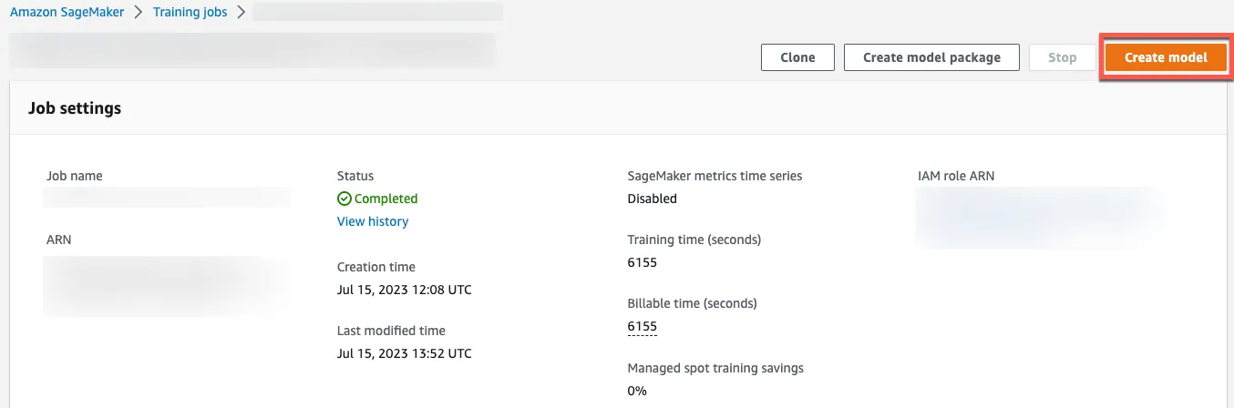
Creating Model from Training Job
Click Create model to create a model from the training job.
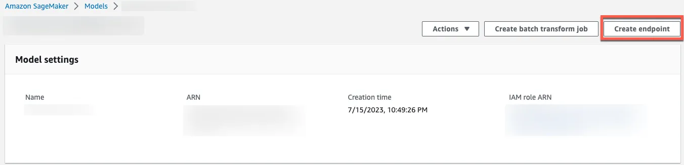
Deploying Model
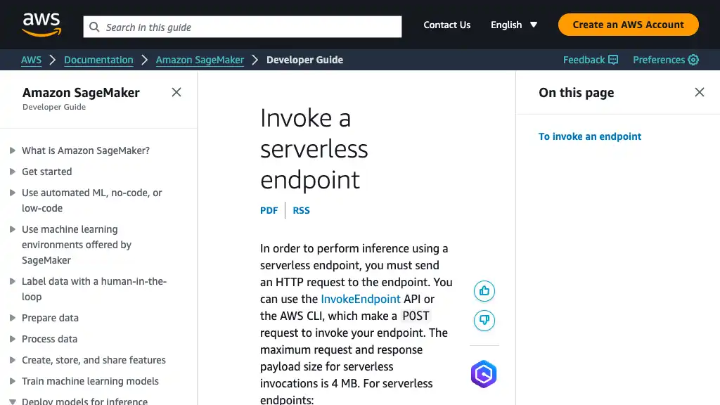
Click Create endpoint to deploy the model from the model page. If you can tolerate cold startup, serverless endpoint should be a better cost-effective choice.
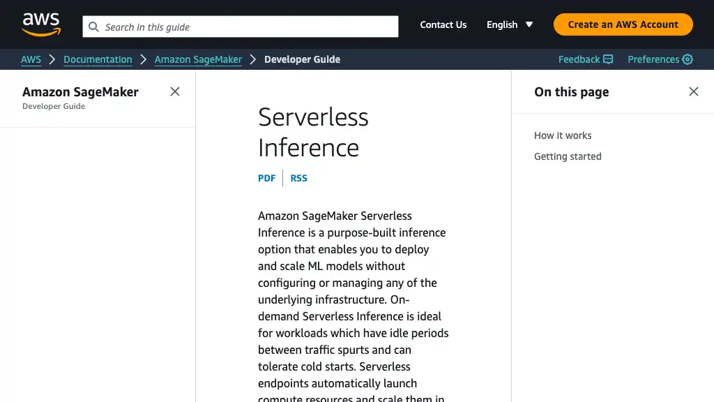
Serverless Inference is a cost-effective option if you have an infrequent or unpredictable traffic pattern. During times when there are no requests, Serverless Inference scales your endpoint down to 0, helping you to minimize your costs.
Making Requests
Using SageMaker Inference Endpoint
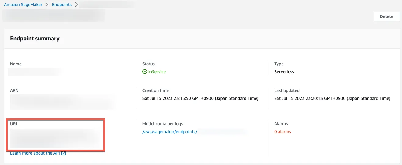
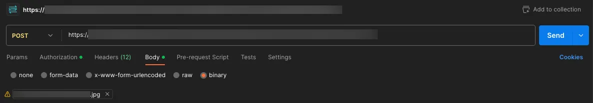
Find the SageMaker inference endpoint in your endpoint detail page. The endpoint can be directly accessed using tools such as curl, Postman, and others.
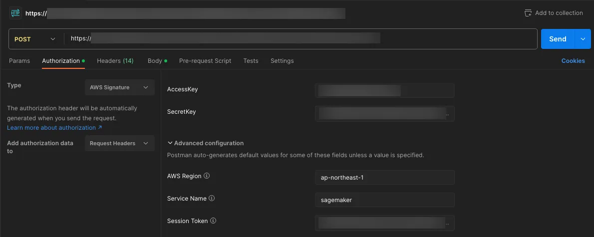
An example image below is using Postman. Specify the following information to provide an AWS Signature V4 header.
- AccessKey
- SecretKey
- Session Token: I strongly recommend using a temporary credential instead of a permanent one.
- AWS Region: Region in which your SageMaker inference endpoint has been started
- Service Name:
sagemaker
Include Accept: application/json header.
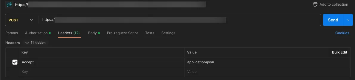
Since the trained model expects binary data as input, provide your image in binary format.
Using AWS SDK (boto3)
You can also use boto3 invoke_endpoint API to perform inference.
import json

import boto3

runtime = boto3.client('sagemaker-runtime')

endpoint_name = '<YOUR_ENDPOINT_NAME>'
content_type = 'application/x-image'
payload = None

# Read an image
with open('/path/to/image.jpg', 'rb') as f:
    payload = f.read()

# Run an inference
response = runtime.invoke_endpoint(
    EndpointName=endpoint_name,
    ContentType=content_type,
    Body=payload
)

# The type of response['Body'] is botocore.response.StreamingBody
# See https://botocore.amazonaws.com/v1/documentation/api/latest/reference/response.html
body = response['Body'].read()

# Print the result
predictions = json.loads(body.decode())
predictions = json.dumps(predictions, indent=2)
print(predictions)

# Write the result to a file
with open('./response.json', 'w') as f:
    f.write(predictions)
Inference Response
Checking Inference Response
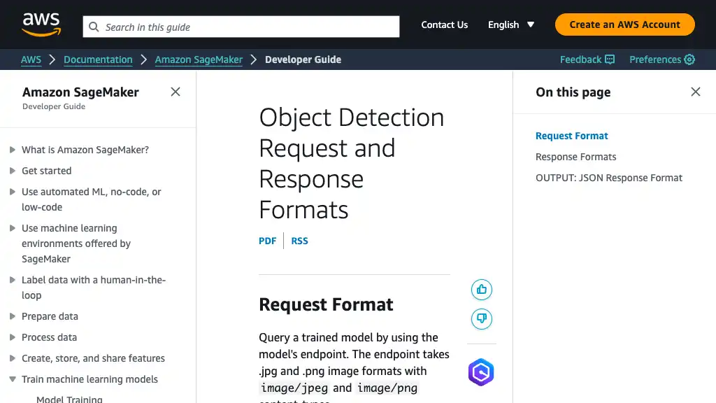
The inference response is in JSON format, including class label IDs, confidence scores, and bounding box coordinates. Please keep it in mind that the bounding box coordinates are relative to the actual image size.
Fore more information about the format, please refer to the official documentation.
{
  "prediction": [
    [
      0.0,
      0.9953756332397461,
      0.3821756839752197,
      0.007661208510398865,
      0.525381863117218,
      0.19436971843242645
    ],
    [
      0.0,
      0.9928023219108582,
      0.3435703217983246,
      0.23781903088092804,
      0.5533013343811035,
      0.6385164260864258
    ],
    [
      0.0,
      0.9911478757858276,
      0.15510153770446777,
...
      0.9990172982215881
    ]
  ]
}
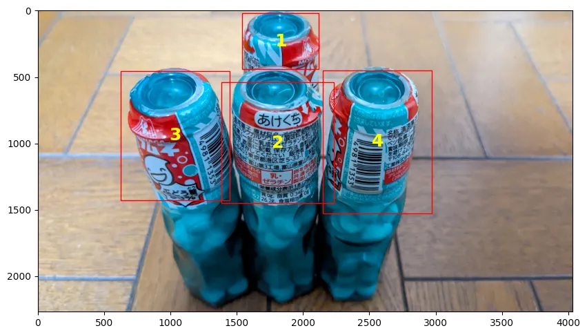
Visualizing Inference Response
To visualize the inference response, this post uses Jupyter Notebook and matplotlib.
import json

import matplotlib.patches as patches
import matplotlib.pyplot as plt
from PIL import Image

# Configure plot
plt.figure()
axes = plt.axes()

# Read an image
im = Image.open('/path/to/image.jpg')
# Display the image
plt.imshow(im)

# Read SageMaker inference predictions
with open('response.json') as f:
    predictions = json.loads(f.read())['prediction']

# Set initial count
count = 0

# Create rectangles
for prediction in predictions:
    score = prediction[1]
    if score < 0.2:
        continue

    # Count up
    count += 1

    x = prediction[2] * im.width
    y = prediction[3] * im.height
    width = prediction[4] * im.width - x
    height = prediction[5] * im.height - y

    rect = patches.Rectangle((x, y), width, height, linewidth=1, edgecolor='r', facecolor='none')
    axes.annotate(count, (x + width / 2, y + height / 2), color='yellow', weight='bold', fontsize=18, ha='center', va='center')
    axes.add_patch(rect)

# Display the rectangles
plt.show()